How to read Execution Plan
When I saw some junior developer writing SQL query, they always busy to get the correct output form there query. Not even thinking about the performance of the query. When they grow up, then they can understand the real fact of performance. It is the key factor of any query execution. How much times it takes to execute. It is going harder to header to learn, how to improve the execution time of a query. I saw many senior people to think about it. The execution time improvement is really a nightmare to us. So, to improve the performance of the query, we must know where we made the mistake and rectify those things that are all.
So I decide to write an article related to execution plan. I try to make it simple that anyone can understand it. Before writing the article, I summarized the facts by reading different articles.
How the execution is happening
To understand the execution plan, we must know how, how the execution is happening. Basically SQL query will be parsed "Top to bottom and Left to right".
Whenever we execute a SQL statement the SQL server will give output by processing the query into two phases.
1. Relational Engine
2. Storage Engine
First the SQL statements will be check against syntax called "Parsing" and the output of this process is in the form of tree called "Sequence Tree". Then the process checks all the table names, columns names, their data types in DML statements and verify against database called "Algebrizer". Then the query process tree goes to the "Query Optimizers", where software will calculate the calculated execution path based on statistics available in the database. Then the optimiser gives some number to each step called "Estimated Cost" for preparation of execution plan. SQL server check the availability of the execution plan is called "Plan Cache". Then the plan will be given to the storage to actually execute the query. It is only the "Estimated execution plan" not the "Actual execution plan". Actual execution plan which will be taken out during the process and stored engine.
The Actual execution plan is cache by stored engine because the plan is used by query engine.
So the "Actual Execution Plan" is more corrects then the "Estimated Execution Plan".
Reading the Execution plan
The graphical plans are read from right to left and from top to bottom. Each icon represents an operation. Some icons are same as estimated and actual execution plan and some are different. Each operator is connected by an arrow that represents the data feed. The thickness of data feed are different, dependent on amount of the data it represents. Thin rows represent the fewer rows and thick one represents more rows.
The SQL Statements
SELECT soh.[SalesOrderID], soh.[OrderDate], soh.[ShipDate], sod.[ProductID],
sod.[OrderQty], sod.[UnitPrice], soh.[CustomerID]
FROM [Sales].[SalesOrderHeader] AS soh
INNER JOIN [Sales].[SalesOrderDetail] AS sod
ON soh.[SalesOrderID] = sod.[SalesOrderID] WHERE soh.[CustomerID] = 29559;
The mentioned SQL statements represent the following execution plan.

Starting at the right and the top you see an Index Seek (NonClustered) against the index named [SalesOrderHeader].[IX_SalesOrderHeader_CustomerId]. This feeds data out to a Nested Loop (Inner Join). Working down we can see a Key Lookup (Clustered) operation against the PK_SalesOrderHeader_SalesOrderID. This is a classic key lookup, or what used to be called, a bookmark lookup. We can see that the data feeds back up to the Nested Loop and then that feeds on down to another Nested Loop operator. Below that is a Clustered Index Seek (Clustered) against the [PK_SalesOrderDetail_SalesOrderId] primary key. Finally the data flow goes out to the SELECT operator. That's the basic information available within the execution plan. Lots more detail is also available.
Hover with the mouse over one of the operators and you will get a tool tip, different for each operation type, showing some of the detail behind the operator. Displayed below is the tool tip for the Key Lookup operator:

At the very top of the tool tip is a description of the operator. In this case, "Uses a supplied clustering key to lookup on a table that has a clustered index." Most operators will include this description, telling you what the operator does within the execution plan. After that, most operations will have a varying number, and type, of fields within the tool tip, supplying different kind of information. An example of one of the common fields is Estimated Operator Cost. You'll see this in most tool tips for most operators. A piece of information that is specific to this operator (although not unique to this operator) is the Seek Predicate information at the bottom of the tool tip.
But the most interesting piece of information for the Key Lookup operator is that it exists within this execution plan. It exists because, while the index on CustomerID is sufficient to get a specific set of rows returned to the application, all the columns needed are not contained on the index. Because the data is stored on the clustered index, and additional set of seeks are required to retrieve the data, which is joined with the information retrieved from the index on CustomerID through the Nested Loop join operation.
To see even more information about the operators in the execution plan, right click an operator and select "Properties" from the drop down menu. This will open a complete properties sheet. Much of the data on the properties sheet is the same as that available in the Tool Tip, but even more is on display in the property sheet.
Show Execution plan displays different type of icons for different takes.
For that please refer to the MSDN. http://msdn.microsoft.com/en-us/library/ms175913.aspx
Hope that the article is quite informative and thanking you to provide your valuable time on it.
When I saw some junior developer writing SQL query, they always busy to get the correct output form there query. Not even thinking about the performance of the query. When they grow up, then they can understand the real fact of performance. It is the key factor of any query execution. How much times it takes to execute. It is going harder to header to learn, how to improve the execution time of a query. I saw many senior people to think about it. The execution time improvement is really a nightmare to us. So, to improve the performance of the query, we must know where we made the mistake and rectify those things that are all.
So I decide to write an article related to execution plan. I try to make it simple that anyone can understand it. Before writing the article, I summarized the facts by reading different articles.
How the execution is happening
To understand the execution plan, we must know how, how the execution is happening. Basically SQL query will be parsed "Top to bottom and Left to right".
Whenever we execute a SQL statement the SQL server will give output by processing the query into two phases.
1. Relational Engine
2. Storage Engine
First the SQL statements will be check against syntax called "Parsing" and the output of this process is in the form of tree called "Sequence Tree". Then the process checks all the table names, columns names, their data types in DML statements and verify against database called "Algebrizer". Then the query process tree goes to the "Query Optimizers", where software will calculate the calculated execution path based on statistics available in the database. Then the optimiser gives some number to each step called "Estimated Cost" for preparation of execution plan. SQL server check the availability of the execution plan is called "Plan Cache". Then the plan will be given to the storage to actually execute the query. It is only the "Estimated execution plan" not the "Actual execution plan". Actual execution plan which will be taken out during the process and stored engine.
The Actual execution plan is cache by stored engine because the plan is used by query engine.
So the "Actual Execution Plan" is more corrects then the "Estimated Execution Plan".
Reading the Execution plan
The graphical plans are read from right to left and from top to bottom. Each icon represents an operation. Some icons are same as estimated and actual execution plan and some are different. Each operator is connected by an arrow that represents the data feed. The thickness of data feed are different, dependent on amount of the data it represents. Thin rows represent the fewer rows and thick one represents more rows.
The SQL Statements
SELECT soh.[SalesOrderID], soh.[OrderDate], soh.[ShipDate], sod.[ProductID],
sod.[OrderQty], sod.[UnitPrice], soh.[CustomerID]
FROM [Sales].[SalesOrderHeader] AS soh
INNER JOIN [Sales].[SalesOrderDetail] AS sod
ON soh.[SalesOrderID] = sod.[SalesOrderID] WHERE soh.[CustomerID] = 29559;
The mentioned SQL statements represent the following execution plan.

Starting at the right and the top you see an Index Seek (NonClustered) against the index named [SalesOrderHeader].[IX_SalesOrderHeader_CustomerId]. This feeds data out to a Nested Loop (Inner Join). Working down we can see a Key Lookup (Clustered) operation against the PK_SalesOrderHeader_SalesOrderID. This is a classic key lookup, or what used to be called, a bookmark lookup. We can see that the data feeds back up to the Nested Loop and then that feeds on down to another Nested Loop operator. Below that is a Clustered Index Seek (Clustered) against the [PK_SalesOrderDetail_SalesOrderId] primary key. Finally the data flow goes out to the SELECT operator. That's the basic information available within the execution plan. Lots more detail is also available.
Hover with the mouse over one of the operators and you will get a tool tip, different for each operation type, showing some of the detail behind the operator. Displayed below is the tool tip for the Key Lookup operator: 
At the very top of the tool tip is a description of the operator. In this case, "Uses a supplied clustering key to lookup on a table that has a clustered index." Most operators will include this description, telling you what the operator does within the execution plan. After that, most operations will have a varying number, and type, of fields within the tool tip, supplying different kind of information. An example of one of the common fields is Estimated Operator Cost. You'll see this in most tool tips for most operators. A piece of information that is specific to this operator (although not unique to this operator) is the Seek Predicate information at the bottom of the tool tip.
But the most interesting piece of information for the Key Lookup operator is that it exists within this execution plan. It exists because, while the index on CustomerID is sufficient to get a specific set of rows returned to the application, all the columns needed are not contained on the index. Because the data is stored on the clustered index, and additional set of seeks are required to retrieve the data, which is joined with the information retrieved from the index on CustomerID through the Nested Loop join operation.
To see even more information about the operators in the execution plan, right click an operator and select "Properties" from the drop down menu. This will open a complete properties sheet. Much of the data on the properties sheet is the same as that available in the Tool Tip, but even more is on display in the property sheet.
Show Execution plan displays different type of icons for different takes.
For that please refer to the MSDN. http://msdn.microsoft.com/en-us/library/ms175913.aspx
Hope that the article is quite informative and thanking you to provide your valuable time on it.
Understanding of Execution Plan [What happened When SQL statement Execute]
Introduction

Performance of query is big factor for every developer. I always put it to higher priority and try to understand the factors behind it. When a T-SQL Query takes a long time to execute, we all say that we must see the execution plan to understand the lack behind it.
As I saw that lot of junior profession cannot understand the execution plan of MS SQL Server properly. So they are unable to find the root cause of the performance lack of a T-SQL query. Here in my blog post we are trying to understand the execution plan properly so that we can understand our query well.
To understand the execution plan is not an easy task and cannot be completed within a single article, so we are thinking to publish it by step by step way with multiple article.
Today is our first session related to understanding of execution plan. In this article we are trying to discuss what happened when we execute a SQL statement.
What happened When SQL statement Execute
To meet the requirement of the query there are two processes that we have to discuss.
1. Process that occurs in the Relational Engine
2. Process that occurs in the Storage Engine
Process that occurs in the Relational Engine
Query Parsing
When the T-SQL query is submitted it checks first that it written correctly or not. This type of syntax checking is called Query parsing. For example if we write a query with SELECTE instead of SELECT the parsing process stop and SQL server returns an Error to the query source.
After successful parsing of a query the output is called the Parse Tree or Query Tree orSequence Tree.
Here we want to mention that the DDL statement is not be Optimized. For example CREATE TABLE/ DROP TABLE etc… So there is only one way to create and drop table and nothing to optimize it.

Algebrizer
The parse tree is passes to a process called Algebrizer. Here it resolves the name of the various object putted in the T-SQL statement. It resolves all the names of the objects, tables and columns, referred to within the query string. It identified Individual columns level, its data type for the objects being accessed. It also determines the location of aggregates (such as GROUP BY, and MAX) within the query, a process called aggregate binding.
This algebrizer process is important because the query may have aliases or synonyms, names that don't exist in the database, that need to be resolved, or the query may refer to objects not in the database. When objects don't exist in the database, SQL Server returns an error from this step, defining the invalid object name.
The algebrizer outputs a binary called the query processor tree, which is then passed on to the query optimizer.
Query Optimizer
The most important pieces of data used by the Query Optimizer are statistics, which MS SQL Server generates and maintains against indexes and columns, explicitly for use by the optimizer.
Using the query processor tree and the statistics, the optimizer applies the model in order to work out what it thinks will be the optimal way to execute the query – that is, it generates anexecution plan.
The Query Optimizer decides if it can access the data through indexes, what types of joins to use and etc. The decisions made by the optimizer are based on what it calculates to be the cost of a given execution plan, in terms of the required CPU processing and I/O. Hence, this is a cost-based plan.
The Query Optimizer generate multiple execution plan and depends on cost basis it choose the best one from them.
The calculation of the Execution cost is the most important calculation for the Query Optimizer and the optimizer will use a process that is more CPU-intensive if it returns results that much faster. If the optimizer thinks that the costing is so high that it cannot give enough time to process and choose the best one, then it can be select less efficient plan also.
If we use a simple select statement from a single table objects without any aggregation or grouping (SELECT * FROM tbl_employee), rather to span time to calculate cost and select the most efficient plan the optimizer use a Trivial plan on it.
SELECT a.empid, a.empname, b.sal
FROM tbl_employee AS a
INNER JOIN tbl_empsal AS b ON a.empid=b.empid
If we add a JOIN clause with this SELECT make the plan non-Trivial and in this case Query optimizer used the cost based calculation to select the plan.
Once the optimizer arrives at an execution plan, the estimated plan is created and stored in a memory space known as the plan cache – although this is all different if a plan already exists in cache. As stated earlier, if the optimizer finds a plan in the cache that matches the currently executing query, this whole process is short-circuited.
Process that occurs in the Storage Engine
Once the Optimizer generates an Execution plan or retrieve it from case, the action switched to the storage engine.
After all the heavy duty work done by optimizer to generate the execution plan, this carefully generated execution plan may be subject to change depends on some criteria
1. MS SQL Server determines that the plan exceeds the threshold for a parallel execution (an execution that takes advantage of multiple processors on the machine).
2. The Statistic that is used to generate the execution plan has been changed.
3. Processes or objects within the query, such as data inserts to a temporary table, result in a recompilation of the execution plan.
Introduction
Performance of query is big factor for every developer. I always put it to higher priority and try to understand the factors behind it. When a T-SQL Query takes a long time to execute, we all say that we must see the execution plan to understand the lack behind it.
As I saw that lot of junior profession cannot understand the execution plan of MS SQL Server properly. So they are unable to find the root cause of the performance lack of a T-SQL query. Here in my blog post we are trying to understand the execution plan properly so that we can understand our query well.
To understand the execution plan is not an easy task and cannot be completed within a single article, so we are thinking to publish it by step by step way with multiple article.
Today is our first session related to understanding of execution plan. In this article we are trying to discuss what happened when we execute a SQL statement.
What happened When SQL statement Execute
To meet the requirement of the query there are two processes that we have to discuss.
1. Process that occurs in the Relational Engine
2. Process that occurs in the Storage Engine
Process that occurs in the Relational Engine
Query Parsing
When the T-SQL query is submitted it checks first that it written correctly or not. This type of syntax checking is called Query parsing. For example if we write a query with SELECTE instead of SELECT the parsing process stop and SQL server returns an Error to the query source.
After successful parsing of a query the output is called the Parse Tree or Query Tree orSequence Tree.
Here we want to mention that the DDL statement is not be Optimized. For example CREATE TABLE/ DROP TABLE etc… So there is only one way to create and drop table and nothing to optimize it.
Algebrizer
The parse tree is passes to a process called Algebrizer. Here it resolves the name of the various object putted in the T-SQL statement. It resolves all the names of the objects, tables and columns, referred to within the query string. It identified Individual columns level, its data type for the objects being accessed. It also determines the location of aggregates (such as GROUP BY, and MAX) within the query, a process called aggregate binding.
This algebrizer process is important because the query may have aliases or synonyms, names that don't exist in the database, that need to be resolved, or the query may refer to objects not in the database. When objects don't exist in the database, SQL Server returns an error from this step, defining the invalid object name.
The algebrizer outputs a binary called the query processor tree, which is then passed on to the query optimizer.
Query Optimizer
The most important pieces of data used by the Query Optimizer are statistics, which MS SQL Server generates and maintains against indexes and columns, explicitly for use by the optimizer.
Using the query processor tree and the statistics, the optimizer applies the model in order to work out what it thinks will be the optimal way to execute the query – that is, it generates anexecution plan.
The Query Optimizer decides if it can access the data through indexes, what types of joins to use and etc. The decisions made by the optimizer are based on what it calculates to be the cost of a given execution plan, in terms of the required CPU processing and I/O. Hence, this is a cost-based plan.
The Query Optimizer generate multiple execution plan and depends on cost basis it choose the best one from them.
The calculation of the Execution cost is the most important calculation for the Query Optimizer and the optimizer will use a process that is more CPU-intensive if it returns results that much faster. If the optimizer thinks that the costing is so high that it cannot give enough time to process and choose the best one, then it can be select less efficient plan also.
If we use a simple select statement from a single table objects without any aggregation or grouping (SELECT * FROM tbl_employee), rather to span time to calculate cost and select the most efficient plan the optimizer use a Trivial plan on it.
SELECT a.empid, a.empname, b.sal
FROM tbl_employee AS a
INNER JOIN tbl_empsal AS b ON a.empid=b.empid
FROM tbl_employee AS a
INNER JOIN tbl_empsal AS b ON a.empid=b.empid
If we add a JOIN clause with this SELECT make the plan non-Trivial and in this case Query optimizer used the cost based calculation to select the plan.
Once the optimizer arrives at an execution plan, the estimated plan is created and stored in a memory space known as the plan cache – although this is all different if a plan already exists in cache. As stated earlier, if the optimizer finds a plan in the cache that matches the currently executing query, this whole process is short-circuited.
Process that occurs in the Storage Engine
Once the Optimizer generates an Execution plan or retrieve it from case, the action switched to the storage engine.
After all the heavy duty work done by optimizer to generate the execution plan, this carefully generated execution plan may be subject to change depends on some criteria
1. MS SQL Server determines that the plan exceeds the threshold for a parallel execution (an execution that takes advantage of multiple processors on the machine).
2. The Statistic that is used to generate the execution plan has been changed.
3. Processes or objects within the query, such as data inserts to a temporary table, result in a recompilation of the execution plan.
Understanding of Execution Plan – II [Reuse of the Execution Plan]
Introduction

Introduction
We promise to our readers that, we are trying to publish a series of article to make the execution plan easier to understand and how to increase the performance of a query by understanding the execution plan. For this we starts our Article named “Understanding of Execution Plan [What happened When SQL statement Execute]”.
If you don’t read it yet or have any doubt please follow the link.
http://www.sqlknowledgebank.blogspot.in/2014/06/understanding-of-execution-plan-what.html
In this article we are trying to discuss about the Reuse of the Execution Plan
Why the Reuse of Execution Plan needs
Why the Reuse of Execution Plan needs
The MS SQL Server takes time to generate the Execution plan depends on the Query that we submit. It can take millisecond, seconds and even minutes also depend on the complexity of the Query submitted by us.
So the MS SQL Server creates the plan and kept in a memory location called Plan Cache or from MS SQL 2005 it is called Procedure Cache, so that SQL Server kept and reuses the Plan whenever possible in order to reduce the overhead.
How it Works
How it Works
Whenever we submit a query to MS SQL server the SQL Server Algebrizer process creates a hash, like a coded signature, of the query. The hash is a unique identifier; its nickname is the query fingerprint.

If a query exists in the cache that matches the query coming into the engine, the entire cost of the optimization process is skipped and the execution plan in the plan cache is reused.
How to Re-Use the Cache
How to Re-Use the Cache
So it is the best practice to write the Query in such way that SQL Server can reuse he plan. To ensure this reuse, it's best to use either stored procedures or parameterized queries. Parameterized queries are queries where the variables within the query are identified with parameters, similar to a stored procedure, and these parameters are fed values, again, similar to a stored procedure.
If, instead, variables are hard coded, then the smallest change to the string that defines the query can cause a cache miss, meaning that MS SQL Server did not find a plan in the cache (even though, with parameterization, there may have existed a perfectly suitable one) and so the optimization process is fired and a new plan created.
When the Cache Plan Removed
When the Cache Plan Removed
MS SQL server never put the plan in Cache forever. They are slowly aged out of the system using an "AGE" formula that multiplies the estimated cost of the plan by the number of times it has been used.
For an example, is a plan with an estimated cost of 10 that has been referenced 5 times has an AGE value of 50.
The lazywriter process, an internal process that works to free all types of cache (including the plan cache), periodically scans the objects in the cache and decreases this value by one each time.
In this following situation the Execution Plan is removed from Memory
Re-Compiling a Execution Plan
The Re-Compiling of an execution plan may be very Expensive Operation and we must remember it. Re-Compilation done in this situation mentioned bellow.
Clearing the Plan from Plan Cache
Sometimes we need to clear the Cache. Suppose we have a bad execution plan in our cache the performance of the Query is so slow and we are unable t improve it due to Bad plan in cache and the plan is not automatically removed.
DBCC FREEPROCCACHE
In this following situation the Execution Plan is removed from Memory
1. When more memory is required by the System
2. The AGE of the Plan is reached to Zero
3. When the plan isn't currently being referenced by an existing connection.
Re-Compiling a Execution Plan
The Re-Compiling of an execution plan may be very Expensive Operation and we must remember it. Re-Compilation done in this situation mentioned bellow.
1. Changing the structure of a Table that is referred by the Query.
2. Changing the Schema of a Table hat is referred by the Query.
3. Changing / Dropping the Index of a Table that is used by Query.
4. Using sp_recompile
5. for tables with triggers, significant growth of the inserted or deleted tables
6. Mixing DDL and DML within a single query, often called a deferred compile
7. Changing the SET options within the execution of the query
Clearing the Plan from Plan Cache
Sometimes we need to clear the Cache. Suppose we have a bad execution plan in our cache the performance of the Query is so slow and we are unable t improve it due to Bad plan in cache and the plan is not automatically removed.
To remove the Plan from Cache we us the following command.
DBCC FREEPROCCACHE
WARNING: Clearing the cache in a production environment
Running it in production environment will clear the cache for all databases on the server. That can result in a significant performance hit because SQL Server must then recreate every single plan stored in the plan cache, as if the plans were never there and the queries were being run for the first time ever.
Understanding of Execution Plan – III - A [ The OPERATORS ]
Introduction

In this article we are mostly focus on the Logical and Physical Operators and try to understand each as it is very important to understand them before understanding the Execution Plan.
The key to understanding execution plans is to start to learn how to understand what the operators do and how this affects your query.
As this tropics is so large we are decide to introduce is part by part.
Different Type of Operators
Each operator has the different type of characteristics, as they manage the memory in different ways. Some operators – primarily Sort, Hash Match (Aggregate) and Hash Join – require a variable amount of memory in order to execute. Because of this, a query with one of these operators may have to wait for available memory prior to execution, possibly adversely affecting performance.
The lists of the operators are mentioned bellow
1. Select (Result)
|
9. Sort
|
17. Spool
|
2. Clustered Index Scan
|
10. Key Lookup
|
18. Eager Spool
|
3. NonClustered Index Scan
|
11. Compute Scalar
|
19. Stream Aggregate
|
4. Clustered Index Seek
|
12. Constant Scan
|
20. Distribute Streams
|
5. NonClustered Index Seek
|
13. Table Scan
|
21. Repartition Streams
|
6. Hash Match
|
14. RID Lookup
|
22. Gather Streams
|
7. Nested Loops
|
15. Filter
|
23. Bitmap
|
8. Merge Join
|
16. Lazy Spool
|
24. Split
|
Most of the operators behave like two was
1. Non-Blocking
2. Blocking
Non-Blocking
A non-blocking operator creates output data at the same time as it receives the input.
A non-blocking operator creates output data at the same time as it receives the input.
Blocking
Blocking operator has to get all the data prior to producing its output. A blocking operator might contribute to concurrency problems, hurting performance.
Blocking operator has to get all the data prior to producing its output. A blocking operator might contribute to concurrency problems, hurting performance.
Queering a Single Table
Here we start a very simple execution plan by Queering a Single Table like
SELECT * FROM Table_Name;
Clustered Index Scan

It occurs when seek against any clustered index or others index can not satisfied. To get the more information about it we have to move the Tool tips. When we look at the bottom of the Tool tip we find the Table Object namedtbl_EMPLOYEERECORD and the Clustered Index namedPK__tbl_EMPL__14CCD97D5D626C84
The Estimated I/O Cost and Estimated CPU Cost are measures assigned by the optimizer, and each operator's cost contributes to the overall cost of the plan.
Indexes in SQL Server are stored in a b-tree. A clustered index not only stores the key structure, like a regular index, but also sorts and stores the data at the lowest level of the index, known as the leaf. This means that a Clustered Index Scan is very similar in concept to a Table Scan. The entire index, or a large percentage of it, is being traversed, row by row, in order to retrieve the data needed by the query.
Why it Occurs
1. Situation when large number of data must be retrieve by the query. For example a Query without any WHERE clause included.
2. When the Statistic of the Index is out of date or incorrect
3. When Query use any Inline Function
Clustered Index Seek

Clustered Index Seek operator occurs when a query uses the index to access only one row, or a few contiguous rows. It's one of the faster ways to retrieve data from the system. We can easily make the previous query more efficient by adding a WHERE clause.
When an index is used in a Seek operation, the key values are used to look up and quickly identify the row or rows of data needed. This is similar to looking up a word in the index of a book to get the correct page number. The benefit of the Clustered Index Seek is that, not only is the Index Seek usually an inexpensive operation when compared to a scan, but no extra steps are required to get the data because it is stored in the index, at the leaf level.
We can see the Tool tip page and see the Ordered property to True.
As in the WHERE clause we use WHERE EMPID=2 but in the Execution plan we can see the WHERE [EMPID] = @1 as it showing the parameter options.
Related Reference
Understanding of Execution Plan – II [Reuse of the Execution Plan]
Summary
In our next level we are going to discuss about more operator one by one. Hope you like it and need your valuable comments related to it.
Understanding of Execution Plan – III - B [ The OPERATORS ]
Introduction

IN my previous Article we just focus about Cluster Index Scan and Clustered Index Seek operators. Continuing my Article series named Understanding of Execution Plan – part III here we are moving with some others operators. Please be focus with our article that you can learn with Execution Plan well.
Non Clustered Index Seek

The operation is a Seek operation against a Non Clustered Index. The operation is effectively no difference with Clustered Index Seek but the only data available is that which is stored in the index itself.
Like a Clustered Index Seek, a Non Clustered Index Seek uses an index to look up the required rows. Unlike a Clustered Index Seek, a Non Clustered Index Seek has to use a non-clustered index to perform the operation. Depending on the query and index, the query optimizer might be able to find all the data in the non-clustered index. However, a non-clustered index only stores the key values; it doesn't store the data. The optimizer might have to look up the data in the clustered index, slightly hurting performance due to the additional I/O required to perform the extra look up.
When Need Covering Index
If the SELECT statement contains some columns of Clustered Index or Any columns that is not a part of non clustered index, in this situation the Non Clustered Index seek cannot be performed an we always get the Clustered Index Scan. To get the Non clustered index Seek we must use the COVERING Index.
CREATE INDEX IX_NONCLUST_EMPNAME ONtbl_EMPLOYEERECORD(EMPNAME)
Property Seek Predicates is important here and we got all information from it.
Key Lookup
A Key Lookup operator is required to get data from the heap or the clustered index, respectively, when a non-clustered index is used, but is not a covering index.

First operation we can see here the Index Seek against the Non clustered Index named IX_NONCLUST_EMPNAME
This is a non-unique, non-clustered index and, in the case of this query, it is non-covering. A covering index is a non-clustered index that contains all of the columns that need to be referenced by a query, including columns in the SELECT list, JOIN criteria and the WHERE clause.
In the tool tips of the Index seek the Output List and Seek Precedence is Important. If we look at the Seek Precedence carefully we find that
Seek Keys[1]: Prefix: [PRACTICE_DB].[dbo].[tbl_EMPLOYEERECORD].EMPNAME = Scalar Operator('Joydeep Das')
As we are using in WHERE Clause EMPNAME = ‘Joydeep Das’
Seek Keys[1]: Start: [PRACTICE_DB].[dbo].[tbl_EMPLOYEERECORD].EMPNAME >= Scalar Operator('Joydeep Das'), End: [PRACTICE_DB].[dbo].[tbl_EMPLOYEERECORD].EMPNAME <= Scalar Operator('Joydeep Das')
If we write LIKE ‘Joydeep%’
Seek Keys[1]: Start: [PRACTICE_DB].[dbo].[tbl_EMPLOYEERECORD].EMPNAME >= Scalar Operator('JoydeeØþ'), End: [PRACTICE_DB].[dbo].[tbl_EMPLOYEERECORD].EMPNAME < Scalar Operator('JoydeeQ')
How it change the code.
[PRACTICE_DB].[dbo].[tbl_EMPLOYEERECORD].EMPID, [PRACTICE_DB].[dbo].[tbl_EMPLOYEERECORD].EMPNAME
Now we look at the tool tips of the Key Lookup on Clustered Index namedPK__tbl_EMPL__14CCD97D5D626C84
Here in the Output list we find
[PRACTICE_DB].[dbo].[tbl_EMPLOYEERECORD].EMPGRADE, [PRACTICE_DB].[dbo].[tbl_EMPLOYEERECORD].SALARY
In Seek Precedence we find
Seek Keys[1]: Prefix: [PRACTICE_DB].[dbo].[tbl_EMPLOYEERECORD].EMPID = Scalar Operator([PRACTICE_DB].[dbo].[tbl_EMPLOYEERECORD].[EMPID])
If this table had been a heap, a table without a clustered index, the operator would have been a RID Lookup operator. RID stands for row identifier, the means by which rows in a heap table are uniquely marked and stored within a table. The basics of the operation of a RID Lookup are the same as a Key Lookup.
Related Reference
Understanding of Execution Plan – II [Reuse of the Execution Plan]
Summary
Introduction
IN my previous Article we just focus about Cluster Index Scan and Clustered Index Seek operators. Continuing my Article series named Understanding of Execution Plan – part III here we are moving with some others operators. Please be focus with our article that you can learn with Execution Plan well.
Non Clustered Index Seek
The operation is a Seek operation against a Non Clustered Index. The operation is effectively no difference with Clustered Index Seek but the only data available is that which is stored in the index itself.
Like a Clustered Index Seek, a Non Clustered Index Seek uses an index to look up the required rows. Unlike a Clustered Index Seek, a Non Clustered Index Seek has to use a non-clustered index to perform the operation. Depending on the query and index, the query optimizer might be able to find all the data in the non-clustered index. However, a non-clustered index only stores the key values; it doesn't store the data. The optimizer might have to look up the data in the clustered index, slightly hurting performance due to the additional I/O required to perform the extra look up.
When Need Covering Index
If the SELECT statement contains some columns of Clustered Index or Any columns that is not a part of non clustered index, in this situation the Non Clustered Index seek cannot be performed an we always get the Clustered Index Scan. To get the Non clustered index Seek we must use the COVERING Index.
CREATE INDEX IX_NONCLUST_EMPNAME ONtbl_EMPLOYEERECORD(EMPNAME)
INCLUDE (EMPID, EMPGRADE, SALARY)
Property Seek Predicates is important here and we got all information from it.
Key Lookup
A Key Lookup operator is required to get data from the heap or the clustered index, respectively, when a non-clustered index is used, but is not a covering index.
First operation we can see here the Index Seek against the Non clustered Index named IX_NONCLUST_EMPNAME
This is a non-unique, non-clustered index and, in the case of this query, it is non-covering. A covering index is a non-clustered index that contains all of the columns that need to be referenced by a query, including columns in the SELECT list, JOIN criteria and the WHERE clause.
Since this index is not a covering index, the query optimizer is forced to not only read the non-clustered index, but also to read the clustered index to gather all the data required to process the query. This is a Key Lookup and, essentially, it means that the optimizer cannot retrieve the rows in a single operation, and has to use a clustered key to return the corresponding rows from a clustered index.
In the tool tips of the Index seek the Output List and Seek Precedence is Important. If we look at the Seek Precedence carefully we find that
Seek Keys[1]: Prefix: [PRACTICE_DB].[dbo].[tbl_EMPLOYEERECORD].EMPNAME = Scalar Operator('Joydeep Das')
As we are using in WHERE Clause EMPNAME = ‘Joydeep Das’
If we write LIKE ‘Joydeep Das’
Seek Keys[1]: Start: [PRACTICE_DB].[dbo].[tbl_EMPLOYEERECORD].EMPNAME >= Scalar Operator('Joydeep Das'), End: [PRACTICE_DB].[dbo].[tbl_EMPLOYEERECORD].EMPNAME <= Scalar Operator('Joydeep Das')
If we write LIKE ‘Joydeep%’
Seek Keys[1]: Start: [PRACTICE_DB].[dbo].[tbl_EMPLOYEERECORD].EMPNAME >= Scalar Operator('JoydeeØþ'), End: [PRACTICE_DB].[dbo].[tbl_EMPLOYEERECORD].EMPNAME < Scalar Operator('JoydeeQ')
How it change the code.
Here from Output List we find the
[PRACTICE_DB].[dbo].[tbl_EMPLOYEERECORD].EMPID, [PRACTICE_DB].[dbo].[tbl_EMPLOYEERECORD].EMPNAME
Now we look at the tool tips of the Key Lookup on Clustered Index namedPK__tbl_EMPL__14CCD97D5D626C84
Here in the Output list we find
[PRACTICE_DB].[dbo].[tbl_EMPLOYEERECORD].EMPGRADE, [PRACTICE_DB].[dbo].[tbl_EMPLOYEERECORD].SALARY
In Seek Precedence we find
Seek Keys[1]: Prefix: [PRACTICE_DB].[dbo].[tbl_EMPLOYEERECORD].EMPID = Scalar Operator([PRACTICE_DB].[dbo].[tbl_EMPLOYEERECORD].[EMPID])
If this table had been a heap, a table without a clustered index, the operator would have been a RID Lookup operator. RID stands for row identifier, the means by which rows in a heap table are uniquely marked and stored within a table. The basics of the operation of a RID Lookup are the same as a Key Lookup.
Related Reference
Understanding of Execution Plan – II [Reuse of the Execution Plan]
Summary
In our next level we are going to discuss about more operator one by one. Hope you like it and need your valuable comments related to it.
Understanding of Execution Plan – III - C [ The OPERATORS ]
Introduction
Contusing the series of my Article related to Understanding of Execution Plan, here we are trying to look some more operations. Hope u can understand it and like it. We need more comments from our readers that all of us can share knowledge and understand the complexity of Execution plan well.
Table Scan
Table Scan occurs with Heap Table only, the table that does not have any clustered index. With clustered Index we can get the Clustered Index Scan which is more or less same as Table scan.
SELECT *
FROM tbl_EMPLOYEERECORD;

The Table Scan occurs for several reasons and the most common is if there is no useful index is there and to retrieve the desired records the query optimizer must search every row. Another common reason is that if we want to retrieve all records from table.
Please remember that, If the table have small number of records then the table scan is not a problem.
RID Lookup
RID Lookup is the heap equivalent of the Key Lookup operation.
As was mentioned in our previous article, non-clustered indexes don't always have all the data needed to satisfy a query. When they do not, an additional operation is required to get that data. When there is a clustered index on the table, it uses a Key Lookup operator. When there is no clustered index, the table is a heap and must look up data using an internal identifier known as the Row ID or RID.
If we specifically filter the results of our previous Database Log query using the primary key column, we see a different plan that uses a combination of an Index Seek and a RID Lookup.
CREATE NONCLUSTERED INDEX IX_NONC_EMPNAME
ON tbl_EMPLOYEERECORD(EMPNAME);
GO
SELECT *
FROM tbl_EMPLOYEERECORD WITH(INDEX(IX_NONC_EMPNAME))
WHERE EMPNAME = 'Joydeep Das';
GO

To return the results for this query, the query optimizer first performs an Index Seek on non clustered index columns on WHERE clauses. While this index is useful in identifying the rows that meet the WHERE clause criteria, all the required data columns are not present in the index.

If we look at the Tool Tip for the Index Seek, we see the value Bmk1000 in the Output List. This Bmk1000 is an additional column, not referenced in the query. It's the key value from the non-clustered index and it will be used in the Nested Loops operator to join with data from the RID Lookup operation.
Next, the query optimizer performs a RID Lookup, which is a type of Bookmark Lookup that occurs on a heap table (a table that doesn't have a clustered index), and uses a row identifier to find the rows to return. In other words, since the table doesn't have a clustered index (that includes all the rows), it must use a row identifier that links the index to the heap. This adds additional disk I/O because two different operations have to be performed instead of a single operation, which are then combined with a Nested Loops operation.

Related Reference
Understanding of Execution Plan – III - B [ The OPERATORS ]
Understanding of Execution Plan – II [Reuse of the Execution Plan]
Summary
In our next level we are going to discuss about more operator one by one. Hope you like it and need your valuable comments related to it.
Understanding the Execution Plan [ When Table JOIN occurs Part-I ]
Introduction
In my previous article we are just using a single table as per our example is concern, Now in this article we are going to see the different table join each other’s and make a single data set by using JOIN. When a JOIN command is issued in T-SQL, it will be resolved through a Join operator. Hope it will be interesting.
How it Works
SELECT e.JobTitle, a.City,
p.LastName + ', ' + p.FirstName AS EmployeeName
p.LastName + ', ' + p.FirstName AS EmployeeName
FROM HumanResources.Employee AS e
INNER JOIN Person.BusinessEntityAddress AS bea
ON e.BusinessEntityID =bea.BusinessEntityID
INNER JOIN Person.Address a ON bea.AddressID =a.AddressID
INNER JOIN Person.Person AS p
ON e.BusinessEntityID = p.BusinessEntityID;
ON e.BusinessEntityID = p.BusinessEntityID;
If we look at the above query the First Name and Last Name is combining together as a meaningful manners. Now we look at the Execution plan.

To read this Execution plan we move from Right to Left. Here we have to identify the most costly operation occurs in the Execution Plan.
1. Index Scan against the Person.Address table (31%).
2. Hash Match join operation between the Person.Person table and the output from the
first Hash Match (21%).
first Hash Match (21%).
3. Other Hash Match join operator between the Person.Address table and the output from
the Nested Loop operator (20%).
the Nested Loop operator (20%).
There are multiple problematic operators in this query since, in general, we're better off with Seek operations instead of Scan operations.

The query optimizer needed to get at the AddressId and the City columns, as shown by the Output List at the bottom of the ToolTip. Please look at the output List of the tooltip of above figure.
The Query optimizer calculates the cost based on Index and statistics of the table objects. Here it takes Actual Number of Rows 19614. That means data was to scan the Index row by row and 19641 rows takes the estimated cost 31% and the total Estimated Operation Cost is 0.158681 (31%).
Here the Estimated Operation Cost means the cost to the Query Optimizer for Executing the specific operation. If Estimated Operation Cost is lower is more efficient the Operation. That does not mean that only seeing the Estimated Operation Cost we decide that it is most expensive operation. We have to calculate other factors also.
What is Has Match Join
In this execution plan we also find the Hash Match Join Operators. First we have to understand what it does.
Hash Match just put two data set into a Temporary Table called Hash Table and use this structure to compare data arrive at the matching set.
Here in our Execution Plan we find two Hash Match join operators. First we find just before SELECT operators (Must read from Right to Left). It just JOIN the output of INDEX SCAN with output of the rest of the operators in the query. This the second most expensive operation in our execution plans. Now we see the tooltip property of this Hash Match Join.

So we have to understand Hash Match, but before that we have to go throw with two concepts called Hashing and Hash Table.
Hashing
It is a programmatic technique where data is converted into symbolic forms for much more efficient searching of data. , SQL Server programmatically converts a row of data in a table into a unique value that represents the contents of the row. We can say it like encryption, a hash value converted to the original data.
Hash Table
It is a data structure and allows quick access to the element. The SQL server take a row from table and hash it into a hash value and store the hash value into a hash table in temp db.
Note: for more information please search on google.
Now move it our main flow, the Hash Match Join operators when SQL server has to join two large datasets. It decides to do so by Hashing the row from the smaller of the two data sets and inserting them into hash table. It then processes the larger data set, one row at a time, against the hash table, looking for matches, indicating the rows to be joined.
If the hash table is relatively small this can be quick in process. If the both table are very large, the hash Match join can be very ineffective in compare to the other type of join. As all the data is stored in the Temp DB, so excessive use of Hash Join in our query provide heavier load of Temp DB.
In our example data from HumanResources.Employee is matched with thePerson.Person table. The Hash Match join occurs well on a Table that are not sorted on JOIN columns means where there is no usable Index. Here in this case MERGE JOIN to work better.
Sending a Hash Match join into execution plan sometimes indicate
1. Missing or Unused Index
2. Missing Where clause
3. A Where clause with Calculation or Conversion
Hare for Hash Match Join we have to investigate our query. That means we have to tune our query by adding Index to make the Join operation more efficient.
Related Reference
Understanding of Execution Plan – III - C [ The OPERATORS]
Understanding of Execution Plan – III - B [ The OPERATORS ]
Understanding of Execution Plan [What happened When SQL statement Execute]
Understanding of Execution Plan – II [Reuse of the Execution Plan]
Summary
In the next level we have to more discuss about our execution plan. So this series will be continued for some more articles. Please be with us.
Understanding the Execution Plan [ When Table JOIN occurs Part-II ]
Introduction
 Continuing my previous article Understanding Execution Plan [ When Table JOIN occurs Part – I ] hare we are describing the others process of Execution Plan.
For reference we again have a look at the Execution plan of the flowing Query.
SELECT e.JobTitle, a.City,
p.LastName + ', ' + p.FirstName AS EmployeeName
ON e.BusinessEntityID = p.BusinessEntityID;

The Nested Loop Join

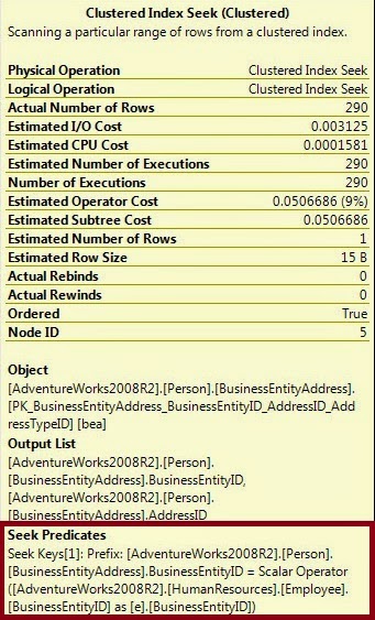
If we look at our Execution Plan carefully we find that the second operation from the top right is a Clustered Index Seek operation (BusinessEntityAddress Table). This is relatively less expensive (only 9%). The Seek is a part of Join Operation and we can see the different search criteria with it. For this we have to look at the Seek Predicates section at the Bottom of the tool tip property.
A Nested Loops join functions by taking a set of data, referred to as the outer set, and comparing it, one row at a time to another set of data, called the inner set. It just likes a cursor, and effectively, it is one but, with the appropriate data set, it can be a very efficient operation.
The data Scan at Employee Table and the Seek against the BusinessEntityAddress table is join at Nested Loop Join operation. To understand it properly we have to look at the tooltip or property of the Nested Loop Join.

We can call Nested Loop as Nested Iteration as the operation takes input from two data sets and join them by scanning from outer data set (Here in our Execution Plan it is the Bottom operator) once for each row in the inner set. If the number of rows is in two data set is small, the Nested Loop operation is much more efficient. As long as the inner data set is small and the outer data set, small or not, is indexed, then this is an extremely efficient join mechanism. Except in cases of very large data sets, this is the best type of join to see in an execution plan.
Related Reference
Introduction
Continuing my previous article Understanding Execution Plan [ When Table JOIN occurs Part – I ] hare we are describing the others process of Execution Plan.
If have you not read my previous article, please go through the following link.
For reference we again have a look at the Execution plan of the flowing Query.
SELECT e.JobTitle, a.City,
p.LastName + ', ' + p.FirstName AS EmployeeName
p.LastName + ', ' + p.FirstName AS EmployeeName
FROM HumanResources.Employee AS e
INNER JOIN Person.BusinessEntityAddress AS bea
ON e.BusinessEntityID =bea.BusinessEntityID
INNER JOIN Person.Address a ON bea.AddressID =a.AddressID
INNER JOIN Person.Person AS p
ON e.BusinessEntityID = p.BusinessEntityID;
ON e.BusinessEntityID = p.BusinessEntityID;
The Nested Loop Join
If we look at our Execution Plan carefully we find that the second operation from the top right is a Clustered Index Seek operation (BusinessEntityAddress Table). This is relatively less expensive (only 9%). The Seek is a part of Join Operation and we can see the different search criteria with it. For this we have to look at the Seek Predicates section at the Bottom of the tool tip property.
A Nested Loops join functions by taking a set of data, referred to as the outer set, and comparing it, one row at a time to another set of data, called the inner set. It just likes a cursor, and effectively, it is one but, with the appropriate data set, it can be a very efficient operation.
The data Scan at Employee Table and the Seek against the BusinessEntityAddress table is join at Nested Loop Join operation. To understand it properly we have to look at the tooltip or property of the Nested Loop Join.
We can call Nested Loop as Nested Iteration as the operation takes input from two data sets and join them by scanning from outer data set (Here in our Execution Plan it is the Bottom operator) once for each row in the inner set. If the number of rows is in two data set is small, the Nested Loop operation is much more efficient. As long as the inner data set is small and the outer data set, small or not, is indexed, then this is an extremely efficient join mechanism. Except in cases of very large data sets, this is the best type of join to see in an execution plan.
Related Reference
Understanding the Execution Plan [ When Table JOIN occurs Part-I ]
http://www.sqlknowledgebank.blogspot.in/2014/10/understanding-execution-plan-when-table.html
Understanding of Execution Plan – III - C [ The OPERATORS]
Understanding of Execution Plan – III - B [ The OPERATORS ]
Understanding of Execution Plan [What happened When SQL statement Execute]
Understanding of Execution Plan – II [Reuse of the Execution Plan]
Summary
http://www.sqlknowledgebank.blogspot.in/2014/10/understanding-execution-plan-when-table.html
| |
Understanding of Execution Plan – III - C [ The OPERATORS]
| |
Understanding of Execution Plan – III - B [ The OPERATORS ]
|
|
Understanding of Execution Plan [What happened When SQL statement Execute]
| |
Understanding of Execution Plan – II [Reuse of the Execution Plan]
|
|
|
|
Summary
In the next level we have to more discuss about our execution plan. So this series will be continued for some more articles. Please be with us.
Understanding the Execution Plan [ When Table JOIN occurs Part-III ]
Introduction
Continuing our journey here we see some others operators exist in our execution plan. Here is the query and Execution Plan that we are working from couple of weeks.
Example Query
SELECT e.JobTitle, a.City,
p.LastName + ', ' + p.FirstName AS EmployeeName
p.LastName + ', ' + p.FirstName AS EmployeeName
FROM HumanResources.Employee AS e
INNER JOIN Person.BusinessEntityAddress AS bea
ON e.BusinessEntityID =bea.BusinessEntityID
INNER JOIN Person.Address a ON bea.AddressID =a.AddressID
INNER JOIN Person.Person AS p
ON e.BusinessEntityID = p.BusinessEntityID;
ON e.BusinessEntityID = p.BusinessEntityID;
Execution Plan

Compute Scalar

First of all it is not a join operation. As it is covered in our Execution Plan, so we must discuss about it. Here we see the properties of the Compute Scalar.

It is represent a operation named Scalar, generally used for calculation purpose. In our case the alias Employeename = ContactLastname + Conatct.FirstName with comma operators between them. If we look at the property, it is not a 0 cost operators (0.001997).
If we look at the property Expr1008 and click at the ellipsis on the right side of the property page this will open the expression.

Related Reference
Understanding the Execution Plan [ When Table JOIN occurs Part-II ]
|
http://www.sqlknowledgebank.blogspot.in/2014/10/understanding-execution-plan-when-table_25.html
|
Understanding the Execution Plan [ When Table JOIN occurs Part-I ]
|
http://www.sqlknowledgebank.blogspot.in/2014/10/understanding-execution-plan-when-table.html
|
Understanding of Execution Plan – III - C [ The OPERATORS]
|
http://www.sqlknowledgebank.blogspot.in/2014/10/understanding-of-execution-plan-iii-c.html
|
Understanding of Execution Plan – III - B [ The OPERATORS ]
|
http://sqlknowledgebank.blogspot.in/2014/10/understanding-of-execution-plan-iii-b.html
|
Understanding of Execution Plan [What happened When SQL statement Execute]
|
http://www.sqlknowledgebank.blogspot.in/2014/06/understanding-of-execution-plan-what.html
|
Understanding of Execution Plan – II [Reuse of the Execution Plan]
|
http://www.sqlknowledgebank.blogspot.in/2014/10/understanding-of-execution-plan-ii.html
|
Understanding of Execution Plan – III - A [ The OPERATORS ]
|
http://www.sqlknowledgebank.blogspot.in/2014/10/understanding-of-execution-plan-iii-the.html
|
Summary
In the next level we have to more discuss about our execution plan. So this series will be continued for some more articles. Please be with us.
 Developers ask a common quest "How to improve the performance of a SQL Query". It is not so easy to answer as lot of factors is related to it. There are some general guidelines that we can follow to improve the overall performance of a query.


Improve the performance by Execution Plan
Introduction
But I recommended the execution plan to understand the performance of the query. I preferred execution plan when I am building the query block step by step.
In this article I am trying to show a basic strategy, how to improve a query by observing the query plan.
Prerequisite
To understand this article, we have a very good knowledge of Index, Index Scan, Index Seek, Table scan etc. Please follow the related tropics of this article, to complete this.
Improving Query
To understand it properly, I am taken an example.
Step-1 [ Creating The Base Table ]
-- Creating the Base Table
IF OBJECT_ID('Emp_Dtls') IS NOT NULL
BEGIN
DROP TABLE Emp_Dtls;
END
GO
CREATE TABLE Emp_Dtls
(EMPID INT NOT NULL IDENTITY,
EMPNAME VARCHAR(50) NOT NULL,
EMPGRADE VARCHAR(1) NOT NULL,
EMPDEPT VARCHAR(30) NOT NULL);
GO
Step-2 [ Inserting the Records ]
DECLARE @i INT=1;
BEGIN TRY
BEGIN TRAN
WHILE (@i <= 50000)
BEGIN
INSERT INTO Emp_Dtls
(EMPNAME, EMPGRADE, EMPDEPT)
VALUES('Developer-'+CONVERT(VARCHAR, @i),'C','DEV');
SET @i=@i+1;
END
SET @i=1;
WHILE (@i <= 50000)
BEGIN
INSERT INTO Emp_Dtls
(EMPNAME, EMPGRADE, EMPDEPT)
VALUES('Devlivery Mgr-'+CONVERT(VARCHAR, @i),'B','DM');
SET @i=@i+1;
END
SET @i=1;
WHILE (@i <= 50000)
BEGIN
INSERT INTO Emp_Dtls
(EMPNAME, EMPGRADE, EMPDEPT)
VALUES('Manager-'+CONVERT(VARCHAR, @i),'A','MGR');
SET @i=@i+1;
END
COMMIT TRAN
END TRY
BEGIN CATCH
ROLLBACK TRAN
END CATCH
Step-3 [ See the Actual Execution Plan ]
-- Execution Plan-1 [ Table Scan ]
SELECT * FROM Emp_Dtls;
As there is NO INDEX defined it going to TABLE SCAN. So the performance of the SQL Query is worst. We have to improve the performance of the Query.
Step-4 [ Create Clustered Index ]
As there is no index over here and the attribute "EMPID" of Table objects "EMP_DTLS" has INTEGER data type, so it is a good candidate key for CLUSTERED INDEX. Now we are going to create the CLUSTERED INDEX on it.
-- Create Custered Index
IF EXISTS(SELECT *
FROM sys.sysindexes
WHERE id = OBJECT_ID('Emp_Dtls')
AND name ='IX_CLUS_Emp_Dtls')
BEGIN
DROP INDEX Emp_Dtls.IX_CLUS_Emp_Dtls;
END
GO
CREATE CLUSTERED INDEX IX_CLUS_Emp_Dtls
ON Emp_Dtls(EMPID);
Aster creating the CLUSTERED INDEX we are going to see the EXECUTION plan again that it Improves or NOT.
-- Execution Plan-2 [ Clustered Index Scan ]
SELECT * FROM Emp_Dtls;
Now we can see that there is Clustered Index Scan. So the performance is little bit improve. At least it uses the CLSUTERED INDEX.
Step-5[ Putting WHERE conditions in Query ]
-- Execution Plan-3 [ Using WHERE Conditions ]
SELECT EMPID, EMPNAME FROM Emp_Dtls WHERE EMPGRADE='A';
As the "EMPGRADE" is used in the WHERE conditions we are going to make a NON CLUSTERED Index on it.
-- Now Create Non Clustered Index on EMPGRADE
IF EXISTS(SELECT *
FROM sys.sysindexes
WHERE id = OBJECT_ID('Emp_Dtls')
AND name ='IX_NONCLUS_EMPGRADE')
BEGIN
DROP INDEX Emp_Dtls.IX_NONCLUS_EMPGRADE;
END
GO
CREATE NONCLUSTERED INDEX IX_NONCLUS_EMPGRADE
ON Emp_Dtls(EMPGRADE);
GO
Now again see the execution plan.
-- Execution Plan-4
SELECT EMPID, EMPNAME FROM Emp_Dtls WHERE EMPGRADE='A';
Here again the clustered Index is used. The non clustered index that we created is not used here. Why?
You can extend the functionality of nonclustered indexes by adding nonkey columns to the leaf level of the nonclustered index. By including nonkey columns, you can create nonclustered indexes that cover more queries.
In this Example the "EMPNAME" is a NONKEY Columns.
Step-6[ Solve the Problem ]
-- Non clustered Index with Incluse
IF EXISTS(SELECT *
FROM sys.sysindexes
WHERE id = OBJECT_ID('Emp_Dtls')
AND name ='IX_NONCLUS_EMPGRADE_EMPNAME')
BEGIN
DROP INDEX Emp_Dtls.IX_NONCLUS_EMPGRADE_EMPNAME;
END
GO
CREATE NONCLUSTERED INDEX IX_NONCLUS_EMPGRADE_EMPNAME
ON Emp_Dtls(EMPGRADE) INCLUDE(EMPNAME);
Now again see the Execution Plan.
-- Execution Plan-5
SELECT EMPID, EMPNAME FROM Emp_Dtls WHERE EMPGRADE='A';
Now the desired output came and it is INDEX SEEK.
Related Tropics